Variational Autoencoders

Autoencoder is a type of neural network that learns a lower dimensional latent representation of input data in an unsupervised manner. The learning task is simple: given an input image, the network will try to reconstruct the image at the output. The loss is measured by the distance between two images, e.g., MSE loss.

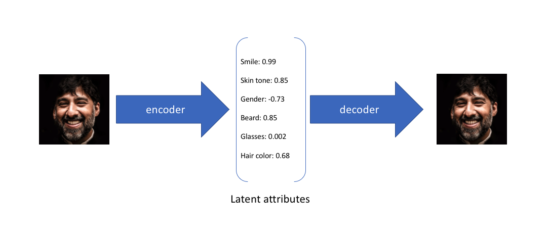
Variational autoencoder improves upon this idea, instead of mapping the inputs to a latent representation using a fixed transformation, variational autoencoder tries to map the inputs to a distribution of latent features. What does that mean? Consider the picture below that illustrates how autoencoder maps the inputs to a latent space:

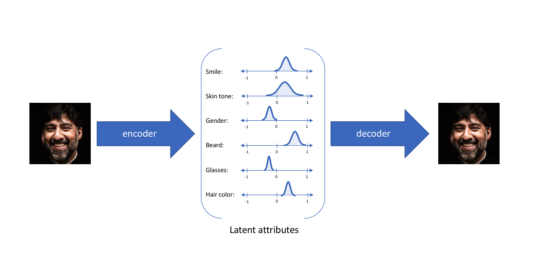
Instead of mapping the inputs to a fixed vector of latent features, VAE maps it to a distribution of latent features:

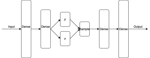
How does VAE map inputs to distributions? VAE assumes each latent features is Gaussian distributed, therefore is network is learning MLP layes that maps the input to a mean $\mu \in \mathcal{R}^d$ and variance $\sigma \in \mathcal{R}^{d \times d}$ where $d$ is the dimensionality of the latent space. VAE then samples a latent representation from this Multivariate Gaussian distribution and feed it to the decoder, which is a determinstic mapping, to reconstruct the input image. The architecture of VAE is shown below:

$\mu$ and $\sigma$ are parameters in the network that can be learned with gradient methods. In order to understand more about VAE, lets now turn to it’s statistical motivation. suppose we have a graphcal model:

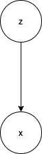
Where there exists some latent variable $z$ that generates $x$. We can only observe $x$ but we would like to know more about $z$. In other words, we would like to compute $p(z|x)$:

However, $p(x) = \int p(x|z) p(z) dz$ is hard to compute and intractable. We can use variational inference and choose a distribution of simpler form (e.g. a family of Gaussian distribution) to approximate this intractable distribution. Let’s define the relationship between the inputs $x$ and the latent encoding vector $z$ by:

prior: $p_{\theta}(z)$

Posterior: $p_{\theta}(z|x)$

Where the distribution is parameterized by $\theta$. Let’s use $q_{\phi}(z|x)$ to approximate the intractable $p_{\theta}(z|x)$. $q_{\phi}(z|x)$ is parameterized by $\phi$. Since we want to use $q_{\phi}(z|x)$ to approximate $p_{\theta}(z|x)$, we want to minimize the KL divergence between $q_{\phi}(z|x)$ and $p_{\theta}(z|x)$:

Expanding the KL divergence term, we have:

$KL(q_{\phi}(z|x) || p_{\theta}(z|x)) = \int q_{\phi}(z|x) \log \frac{q_{\phi}(z|x)}{p_{\theta}(z|x)} dz$

$= \int q_{\phi}(z|x) \log \frac{q_{\phi}(z|x) p_{\theta}(x)}{p_{\theta}(z, x)} dz = \int q_{\phi}(z|x) (\log p_{\theta}(x) + \log \frac{q_{\phi}(z|x)}{p_{\theta}(z, x)})dz$

$= \log p_{\theta}(x) + \int q_{\phi}(z|x) \log \frac{q_{\phi}(z|x)}{p_{\theta}(z, x)}dz$

Rearranging the terms above, we have:

Or:

Where the LHS is a constant (the log likelihood of the data is constant), on the RHS, the KL divergence term is what we are trying to minimize. Instead of minimizing KL divergence term, we can maximizing the second term $\int q_{\phi}(z|x) \log \frac{p_{\theta}(z, x)}{q_{\phi}(z|x)}dz$, which is called the variational lower bound, which we will denote as $\mathcal{L}$. The reason $\mathcal{L}$ is called the variational lower bound is because the KL divergence term is non-neggative, therefore $\mathcal{L}$ is a lower bound of the log likelihood $log p_{\theta}(x)$. A different way to look at this optimization problem is that since $\mathcal{L}$ is a lower bound of the log likelihood, maximizing the lower bound also maximizes the log likelihood itself.

If we further expand the variational lower bound $\mathcal{L}$, we have:

$\mathcal{L} = \int q_{\phi}(z|x) \log \frac{p_{\theta}(z, x)}{q_{\phi}(z|x)}dz = \int q_{\phi}(z|x) \log \frac{p_{\theta}(x|z)p_{\theta}(z)}{q_{\phi}(z|x)}dz$

$= \int q_{\phi}(z|x) \log p_{\theta}(x|z)dz - \int q_{\phi}(z|x) \log \frac{q_{\phi}(z|x)}{p_{\theta}(z)}dz$

$= E_{z \sim q_{\phi}(z|x)} [\log p_{\theta}(x|z)] - KL(q_{\theta}(z|x) || p_{\theta}(z))$

Since the decoder network is determinstic, we can write the first term as:

$E_{z \sim q_{\phi}(z|x)} [\log p_{\theta}(x|z)] = E_{z \sim q_{\phi}(z|x)} [\log p_{\theta}(x|\hat{x})]$

If we assume $p_{\theta}(x|\hat{x})$ has the from of: $p_{\theta}(x|\hat{x}) = e^{-(x-\hat{x})^2}$, the log likelihood would become maximizing the negative MSE loss between the input and the reconstruction:

$\mathcal{L} = -(x-\hat{x})^2 - KL(q_{\theta}(z|x) || p_{\theta}(z))$

If we assume both the prior $p_{\theta}(z)$ and posterior approximation $q_{\phi}(z|x)$ are Gaussian, the KL divergenceterm can be intergrated analutically:

Let $J$ be the dimension of latent representation $z$:

$- KL(q_{\theta}(z|x) || p_{\theta}(z)) = \frac{1}{2} \sum_{j=1}^J (1 + \log((\sigma_j^2)) - (\mu_j^2) - (\sigma_j^2))$

Therefore, the loss function for VAE is:

$\mathcal{l} = (x-\hat{x})^2 - \frac{\beta}{2} \sum_{j=1}^J (1 + \log((\sigma_j^2)) - (\mu_j^2) - (\sigma_j^2))$

Where $\beta$ is the coefficient for the regularizer.

Now, let’s see how VAE performs in practice. We will implement and experiment VAE in Python. I used PyTorch to implement the VAE. First, let’s load all the neccessary libraries:

import numpy as np
import torch
import matplotlib.pyplot as plt
import matplotlib
from numpy import linalg as LA
import torch.nn as nn
import torch.nn.functional as F
import torchvision
from torchvision import transforms, datasets
import torch.optim as optim
from PIL import Image
import os
from mpl_toolkits.axes_grid1 import ImageGrid

Now let’s implement a PyTorch layer that takes a mean $\mu$ and variance $\sigma$ and samples from the Gaussian distribution. Since sampling is not differentiable, we will use the “reparametrization trick”. That is, instead of sampling from a Gaussian distribution, we will use a determinstic function to output the sample:

where $\epsilon \in \mathcal{N}(0, I)$. We call this layer Gaussian sample layer:

class gaussian_sample_layer(nn.Module):

    def __init__(self, latent_dim):
        super(gaussian_sample_layer, self).__init__()
        self.latent_dim = latent_dim
        self.L = 1
        
    def forward(self, mu, sigma):
        epsilon_dist = torch.distributions.MultivariateNormal(torch.zeros(self.latent_dim),torch.eye(self.latent_dim))
        epsilon = epsilon_dist.sample((self.L,))
        epsilon = torch.sum(epsilon, dim=0) / self.L
        a = mu + epsilon * sigma
        return a

And we implement the VAE network using only $2$ latent dimensions:

class variational_autoencoder(torch.nn.Module):

    def __init__(self):
        super(variational_autoencoder, self).__init__()
        input_size = 784
        output_size = 784
        self.latent_dim = 2
        self.mlp1 = nn.Linear(input_size, 128)
        self.mu = nn.Linear(128, self.latent_dim)
        self.sigma = nn.Linear(128, self.latent_dim)
        self.gaussian = gaussian_sample_layer(self.latent_dim)
        self.mlp4 = nn.Linear(self.latent_dim, 128)
        self.out = nn.Linear(128, output_size)
        self.batch_size = 8

    def forward(self, x):
        h1 = F.sigmoid(self.mlp1(x))
        mu = F.sigmoid(self.mu(h1))
        sigma = F.sigmoid(self.sigma(h1))
        z = self.gaussian(mu, sigma)
        h4 = F.tanh(self.mlp4(z))
        y_hat = F.relu(self.out(h4))
        return y_hat, mu, sigma
    
    def loss(self, x, y, beta=0.0001):
        y_hat, mu, sigma = self.forward(x)
        c = nn.MSELoss()
        l = c(y_hat, y) - beta * 1/2 * torch.sum(1 + torch.log(sigma**2) - mu**2 - sigma**2)
        return l
    
    def decoder(self, x):
        f = F.relu(self.out(F.tanh(self.mlp4(x))))
        return f

Now let’s load the training set:

batch_size = 8
train = datasets.MNIST(root='./data', train=True, download=True, transform=transforms.Compose([transforms.ToTensor()]))
trainset = torch.utils.data.DataLoader(train, batch_size=batch_size, shuffle=True)

And initialize a VAE instance and begin training:

vae = variational_autoencoder()
optimizer = optim.Adam(vae.parameters(), lr=3e-4)
for epoch in range(100):
    cnt = 0
    l = 0
    for data in trainset:
        data = data[0].squeeze()
        x = torch.reshape(data, (batch_size, 784))
        y = x.clone()
        optimizer.zero_grad()
        y_hat, _, _ = vae(x)
        loss = vae.loss(x, y)
        loss.backward()
        optimizer.step()
        l += loss
        cnt += 1
    print(l)

Now let’s load the testset and see the model’s ability to reconstruct the images:

test = datasets.MNIST(root='./data', train=False, download=True, transform=transforms.Compose([transforms.ToTensor()]))
testset = torch.utils.data.DataLoader(test, batch_size=batch_size, shuffle=True)

And now produce a 20 $\times$ 20 grid to show the reconstruction:

results = []
cnt = 0
pairs_per_row = 10
for test in testset:
    if cnt == pairs_per_row ** 2:
        break
    data = test[0].squeeze()
    x = torch.reshape(data, (batch_size, 784))
    out = vae(x)[0].detach().numpy()
    cnt += 1
    for i in range(data.shape[0]):
        results.append(data[i])
        results.append(out[i].reshape(28, 28))
    cnt += 1
    
fig = plt.figure(figsize=(16, 16.))
grid = ImageGrid(fig, 111, nrows_ncols=(pairs_per_row*2, pairs_per_row*2), axes_pad=0.1,)

for ax, im in zip(grid, results):
    ax.imshow(im, cmap='gray')

The results are:

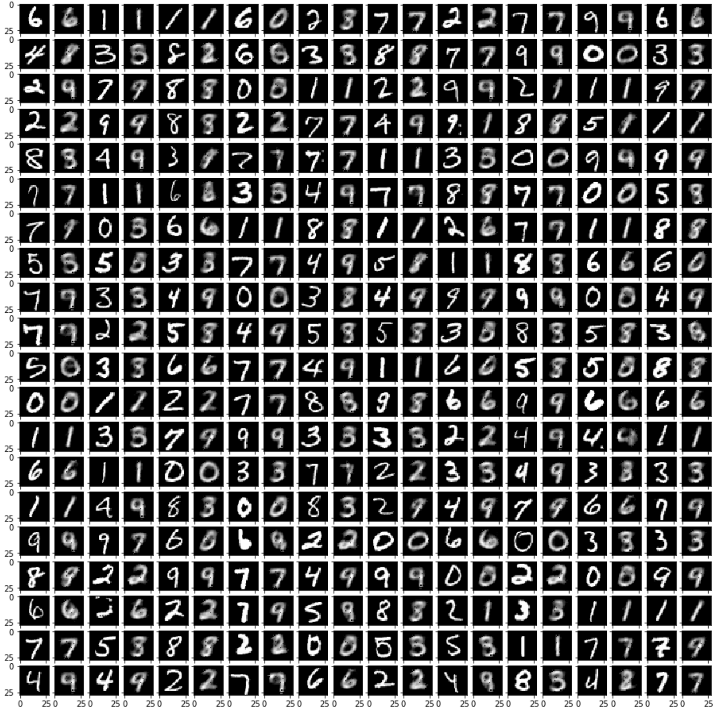
As we can see, the reconstruction is different from reconstructions made by traditional autoencoders. A lot of the reconstructed digits are having different writing styles (different strokes, diffent turns and twists, etc.). Therefore we can deduct that the latent space distribution is characterizing the features of inputs in terms of distribution, not a fixed form mapping.

Now, let’s create a grid of values between $[0, 1]$ in 2D and see what sample does the decoder maps them to:

steps = 20
x = np.linspace(0, 1, num=steps)
y = np.linspace(0, 1, num=steps)
z = []
for xval in x:
    for yval in y:
        z.append((xval, yval))
z = np.array(z)

imgs = []
for pair in z:
    cnt += 1
    imgs.append(vae.decoder(torch.from_numpy(pair).float()).detach().numpy().reshape(28, 28))

fig = plt.figure(figsize=(16, 16.))
grid = ImageGrid(fig, 111, nrows_ncols=(steps, steps), axes_pad=0.1,)

for ax, im in zip(grid, imgs):
    ax.imshow(im, cmap='gray')

The results are:

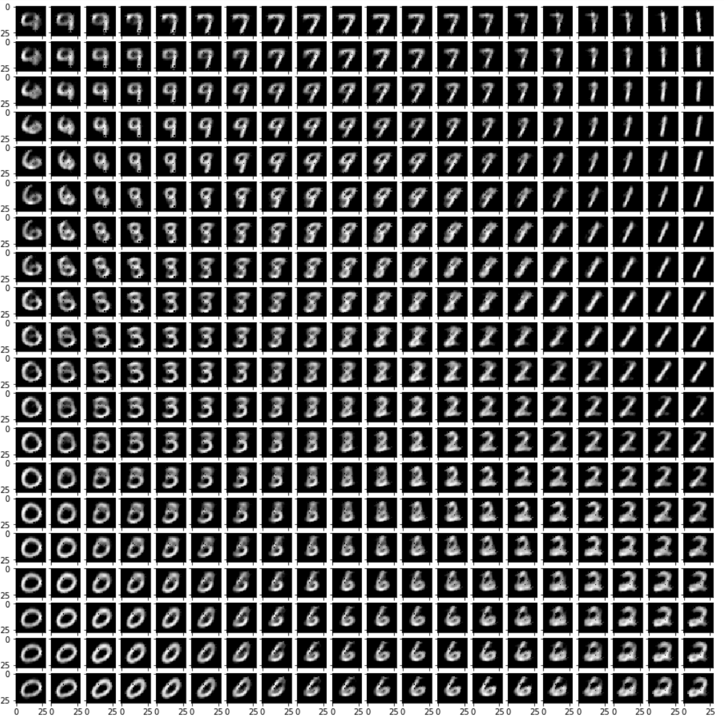
Which is really interesting. First of all, the neighbors are really similar to each other and it’s slowly morphing into different classes; second of all, since VAE is learning a distribution, there are some obvious overlapping between similar classes (4 and 9 and overlapping, 3, 5 and 8 are overlapping).

This blog is based on the paper Auto-Encoding Variational Bayes.

The Jupyter Notebook of the code can be found here.

Thank you for reading!