Finite-dimensional Approximation of Kernel SVM with Random Fourier Features

Support vector machines are in my opinion the best machine learning algorithm. It generalizes well with less risk to overfitting, it scales well to high-dimensional data, and kernel trick makes it possible to efficiently lift the feature space to higher dimensions, and the optimization problem for SVMs are usually quadratic programs that are efficient to solve and has a global minimum. However, there are a few drawbacks to SVMs. The biggest one is that it doesn’t scale well with large dataset and the inference time depends on the size of the training dataset. For a training set of set $m$, where $x \in \mathcal{R}^d$, the time complexity to compute the gram matrix is $\mathcal{O}(m^2 d)$ and the time complexity to for inference is $\mathcal{O}(md)$. This time complexity scales poorly with large training sets.

To address this issue, we can approximate the kernel functions using finite-dimensional appromixation. That is, we can explicitly map the data to a low-dimensional Euclidean inner product space using a randomized feature map $z: \mathcal{R}^d \to \mathcal{R}^D$ so that the inner product between pairs of transformed points approximates their kernel evaluation: $k(x, y) = \langle \phi(x) \phi(y) \rangle \approx z(x)’z(y)$.

Unlike the lifting $\phi(\cdot)$, $z(\cdot)$ is low-dimensional, therefore we can just simply transform the input with $z(\cdot)$, and then use fast linear methods to approximate the answer of the corresponding nonlinear kernel machine.

The finite-dimensional approximation only works for approximating shift invariant kernels, that is, kernel functions whose value only depends on the difference between two points $x$ and $y$. Popular kernel functions such as Gaussian kernels and Laplacian kernels are all shift invariant kernels.

How to approximate a nonlinear kernel function with potentially infinite dimensions using finite-dimensional mapping? The following classic theorem from harmonic analysis is the foundation for this transformation:

Bochner. A continuous kernel $k(x, y)=k(x-y)$ on $\mathcal{R}^d$ is positive definite if and only if $k(\delta)$ is the Fourier transform of a non-negative measure.

That is, if a shift-invariant kernel $k(\delta)$ is properly scaled, Bochner’s theorem guarantees that its Fourier transform $p(\omega)$ is a proper probability distribution. Let $\zeta_{\omega}(x) = e^{j\omega’ x}$:

And $\zeta_{\omega}(x)\zeta_{\omega}(y)^{*}$ is an unbiased estimate of $k(x, y)$ when $\omega$ is drawn from $p$. According to Ali Rahimi el.al., (1) converges when the complex exponentials are replaced with cosines. Therefore, we obtain a real-valued mapping that satisfies the condition $E[ \zeta_{\omega}(x)\zeta_{\omega}(y)] = k(x, y)$ by setting $z_{\omega}(x) = \sqrt{2} cos(\omega’x+b)$ where $\omega$ is drawn from $p(\omega)$ and $b$ is drawn uniformaly from $[0, 2\pi]$

To make the approximate $\zeta_{\omega}(x)\zeta_{\omega}(y)$ closer to the target value (its mean) $k(x, y)$, we need to sample it multiple times and take the average. Let $D$ be the number of samples we take, which is also the number of finite dimension we wish to approximate the kernel function with, we define a mapping $z(\cdot): \mathcal{R}^d \to \mathcal{R}^D$:

and we apply linear SVM to the transformed data.

Now lets apply this technique in Python. First, we create a good sampling method for sampling $\omega$ from $p(\omega)$:

def metropolis_hastings(p, dim, iter=1000):
    x = np.zeros(dim)
    samples = np.zeros((iter, dim))

    for i in range(iter):
        x_next = x + np.random.multivariate_normal(np.zeros(dim), np.eye(dim))
        if np.random.rand() < p(x_next) / p(x):
            x = x_next
        samples[i] = x

    return samples

This is Metropolis Hastings algorithm, it’s a type of MCMC sampling method. Now, lets create the functions that computes the Fourier transforms of Gaussian kernels and Laplacian kernels:

def gaussian_fourier(w):
    return (2*np.pi)**(-w.shape[0]/2) * np.exp(-LA.norm(w)/2)

def laplacian_fourier(w):
    p = 1
    for i in range(w.shape[0]):
        p *= 1 / (np.pi * (1 + w[i]))
    return p

I coded a $random_fourier_features_svm$ class that trains on Fourier features drawn from corresponding Fourier transforms of different kernel functions:

class random_fourier_features_svm:
    def __init__(self, kernel_fourier=gaussian_fourier, D=500):
        self.kernel_fourier = kernel_fourier
        self.D = D
        
    def _feature_mapping(self, X, omega, bias):
        X_map = np.zeros((X.shape[0], self.D))
        for i in range(X.shape[0]):
            for j in range(self.D):
                X_map[i, j] = np.cos(np.dot(omega[j], X[i]) + bias[j]) * np.sqrt(2/self.D)
        return X_map
    
    def _draw_features(self, d, max_iter=1000):
        s = metropolis_hastings(self.kernel_fourier, dim=d, iter=max_iter)
        omega = s[np.random.randint(low=10, high=max_iter, size=self.D)]
        bias = np.random.uniform(low=0, high=2*np.pi, size=self.D)
        self.omega = omega
        self.bias = bias
        
    def fit(self, X_train, y_train, max_iter=1000, C=10):
        d = X_train.shape[-1]
        self._draw_features(d, max_iter=max_iter)
        X_train_map = self._feature_mapping(X_train, self.omega, self.bias)
        m,n = X_train_map.shape
        y_train = y_train.reshape(-1,1) * 1.
        K = np.dot(X_train_map, X_train_map.T)
        H = np.outer(y_train, y_train) * K
        
        P = matrix(H)
        q = matrix(-np.ones(m))
        G = matrix(np.vstack((np.eye(m)*-1,np.eye(m))))
        h = matrix(np.hstack((np.zeros(m), np.ones(m) * C)))
        A = matrix(y_train, (1, m))
        b = matrix(0.)

        #Run solver
        sol = solvers.qp(P, q, G, h, A, b)
        alphas = np.array(sol['x'])

        alphas = alphas.reshape(alphas.shape[0])

        sup_vec_idx = np.argwhere(np.logical_or(alphas > 1e-4, alphas < -1e-4))
        sup_vec_idx = sup_vec_idx.reshape(sup_vec_idx.shape[0])
        X_sup_vec = X_train_map[sup_vec_idx]
        y_sup_vec = y_train[sup_vec_idx]
        alphas_sup_vec = alphas[sup_vec_idx]
        
        w = np.zeros(self.D)
        for i in range(alphas_sup_vec.shape[0]):
            w += alphas_sup_vec[i] * y_sup_vec[i] * X_sup_vec[i]
        b = - (np.max(np.dot(X_train_map[np.where(y_train == -1)[0]], w)) + np.min(np.dot(X_train_map[np.where(y_train == 1)[0]], w))) / 2
        self.w = w
        self.b = b
        self.sup_vec_idx = sup_vec_idx
        
    def evaluate(self, X_test, y_test):
        X_test_map = self._feature_mapping(X_test, self.omega, self.bias)
        return np.sum((np.sign(np.dot(X_test_map, self.w) + self.b) == y_test).astype("int")) / X_test_map.shape[0]

Where the training data are mapped using $z(x)$ defined above to dimension $D$, and the kernel is a linear kernel, that is, the gram matrix is computed as: $K = X X^T$ where $X \in \mathcal{R}^{m\times d}$ is the training set. The training process indentifies the support vectors and compute the weight vector $w$ according to the representer theorem: $w=\sum_{s \in S} \alpha[s] y[s] X[s]$ where $w \in \mathcal{R}^D$ and $S$ is set of indices of support vectors. To make a prediction on a new test data $x$, we just simply need to apply linear computation: $\hat{y} = sign(w^T x)$. The new inference complexity reduces to $\mathcal{O}(D)$ which is a lot more attrative than $\mathcal{O}(m d)$.

How does this Random Fourier features SVM work in practice? The answer is it works just as well if not better than the vanilla SVM. Here are some experiment results:

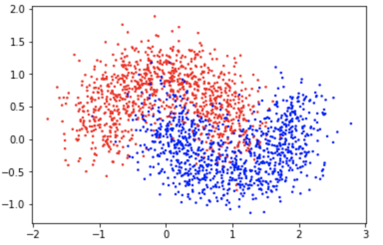
X, y = make_moons(n_samples=2000, noise=0.3)
colors = ['red','blue']
plt.scatter(X[:, 0], X[:, 1], c=y, cmap=matplotlib.colors.ListedColormap(colors), s=2)
y[y == 0] = -1
seed = 1
X_train, X_test, y_train, y_test = train_test_split(X, y, test_size=0.2, random_state=seed)

This is a two-moon dataset with a significant amount of noise($0.3$):

We train on the training set and evaluate on the test set:

clf = random_fourier_features_svm()
clf.fit(X_train, y_train)
clf.evaluate(X_test, y_test)

The accuracy is pretty high for such a noisy dataset.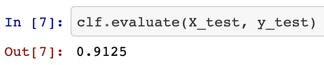

And now let’s visualize the support vectors:

X_sup_vec_original = X_train[clf.sup_vec_idx]
X_non_sup_vec = X_train[~np.isin(np.arange(len(X_train)), clf.sup_vec_idx)]
y_non_sup_vec = y_train[~np.isin(np.arange(len(y_train)),clf. sup_vec_idx)]
y_non_sup_vec = y_non_sup_vec.reshape(y_non_sup_vec.shape[0])
fig, ax = plt.subplots()
colors = ['red','blue']
ax.scatter(X_sup_vec_original[:, 0], X_sup_vec_original[:, 1], c="black", s=6, marker='x', label="Support Vectors")
ax.scatter(X_non_sup_vec[:, 0], X_non_sup_vec[:, 1], c=y_non_sup_vec, cmap=matplotlib.colors.ListedColormap(colors), s=2)
ax.legend(loc="upper right")
plt.show()

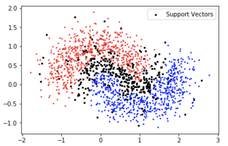
Which looks a lot like the polynomial kernel support vector formations.

The code is available in this jupyter notebook.

Thanks for reading!