Learning with Invariance using Tangent Distance Kernel

In kernel SVM, most kernel functions relies on some distance metric. A commonly used distance metric is the Euclidean distance. However in fields like pattern recognition, Euclidean distance is not robust to simple transformations that don’t change the class label: rotation, translation and scaling. For example:

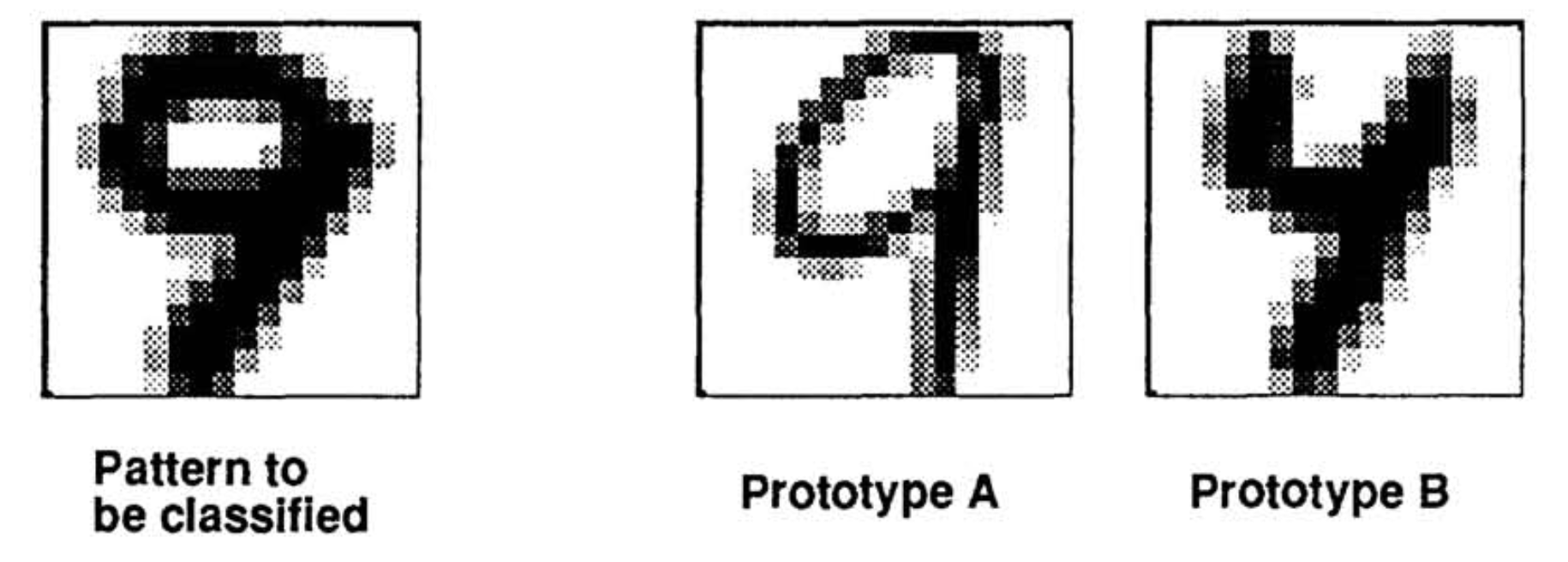
According to Euclidean distance B is closer than A. A better distance metric would argue that A is closer than B. Distance metrics that are robust to invariances that don’t alter class labels are extremely important to distance-based classifiers like nearest neighbor classifier and support vector machines.

When pattern $P$ is transformed with a transformation $s$ that depends on a parameter $\alpha$ (e.g. rotation of the angle, step of the translation, of the magnitude of the scaling), the set of all transformed points $S_P = {x \vert \forall \vec{\alpha} s.t. x = s(\vec{\alpha}, P)} $ where $s(\vec{\alpha}, P)$ defines a differentiable tranformation, form a manifold in vector space of the inputs. Note that $s(0, x) = x$.

Therefore, an invariant distance metric should measure the minimum distance between the two manifolds formed by their respective set of all transformed points $S_P$. However, the minimum distance between two manifolds is hard to calculate, therefore we will approximate that distance using the tangent distance. To summerize: we will approximate the distance betwenn two manifolds induced by point $x$ and $x’$ using x’s distance to the tangent line of the manifold induced by $x’$ at x’. To illustrate this in picture:

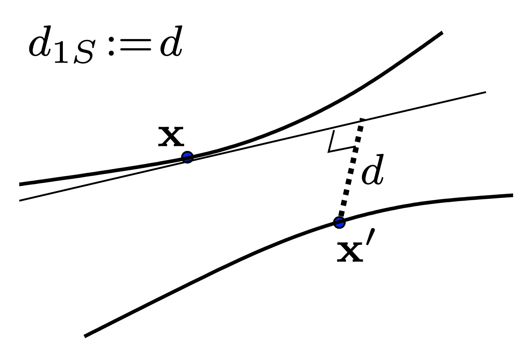
The dash line is the tangent distance. The illustrated distance, called a one sided tangent distance, is obtained through the following optimization problem:

where $L$ is the tangent line of the manifold induced by $x$ at point $x$ and is defined mathematically as: $L = \left.\frac{\partial s(\vec{\alpha}, x)}{\partial \vec{\alpha}}\right \vert_{\vec{\alpha}=0}$

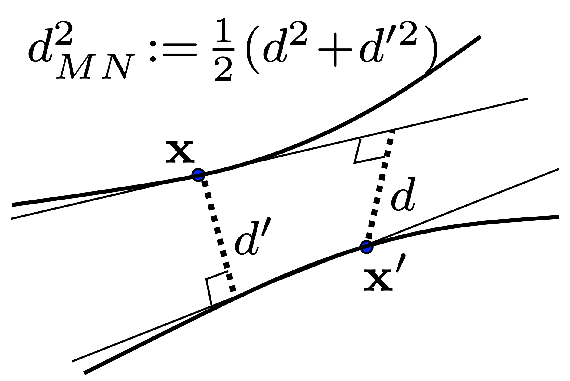
You might notice that this distance is not symmetric, we can define a symmetric version using $d_{1S}(x, x’)$: $d_{MN}(x, x’) := \sqrt{\frac{1}{2} (d_{1S}^2(x, x’) + d_{1S}^2(x’, x))}$, which is called the square of the mean tangent distance. The symmetric tangent distance is illustrated below:

Tangent distance is not an actual distance metric like the Euclidean distance since it doesn’t satisfy the trianglar ineuqality.

Now let’s see some experiment results. In this experiment, I calculated the tangent vector $L$ (the direction of the tangent line of the manifold at point $x$) by $\frac{s(-\delta, x) - s(\delta, x)}{2\delta}$ where $\delta$ is a small rotation angle:

def rotation_deritavtive(x):
    h,w = x.shape
    delta = 15
    M1 = cv2.getRotationMatrix2D(((w-1)/2.0,(h-1)/2.0), -delta, 1)
    M2 = cv2.getRotationMatrix2D(((w-1)/2.0,(h-1)/2.0), delta, 1)
    return ((cv2.warpAffine(x, M1, (w,h)) - cv2.warpAffine(x, M2, (w,h))) / delta*2).reshape(x.shape[0]*x.shape[-1], 1)

I fixed $\delta=15$ which is a fairly small rotation. The one sided tangent distance is calculated as:

def one_side_min_tangent_dist(x1, dx1, x2, learning_rate=0.0005, max_iter=5000, delta=0.0001):
    d, r = dx1.shape
    a = np.random.random((r,1))
    t = 0
    while True:
        b = copy.copy(a)
        a = a - learning_rate * np.dot((x1 + np.dot(dx1, a) - x2).T, dx1)
        t += 1
        if np.sqrt(np.mean((b-a)**2)) < delta or t > max_iter:
            break
    return np.sqrt(np.mean((x1 + np.dot(dx1, a) - x2)**2)) 

Where the function is performing gradient descent to obtain the minimum tangent distance. Then the symmetric tangent distance function can be constructed as:

def tangent_dist(x1, x2):
    dx1 = rotation_deritavtive(x1)
    dx2 = rotation_deritavtive(x2)
    x1 = x1.reshape(x1.shape[0]*x1.shape[-1], 1)
    x2 = x2.reshape(x2.shape[0]*x2.shape[-1], 1)
    d1s_x1_x2 = one_side_min_tangent_dist(x1, dx1, x2)
    d1s_x2_x1 = one_side_min_tangent_dist(x2, dx2, x1)
    return np.sqrt(1/2 * (d1s_x1_x2**2 + d1s_x2_x1**2))

Now we define a simple function that performs the rotation of the images using the cv2 libary:

def rotate_image(image, angle):
    center = tuple(np.array(image.shape[1::-1]) / 2)
    rot_mat = cv2.getRotationMatrix2D(center, angle, 1.0)
    result = cv2.warpAffine(image, rot_mat, image.shape[1::-1], flags=cv2.INTER_LINEAR)
    return result

now we can compare the effects of rotations on Euclidean distance and tangent distance:

tanh_dist = []
euclidean_dist = []
rotation_max = 30
for i in range(-rotation_max, rotation_max, 5):
    x = trainX[12]
    xr = rotate_image(x, -i)
    x = x/255
    xr = xr/255
    tanh_dist.append(tangent_dist(x, xr))
    euclidean_dist.append(np.sqrt(np.mean((x - xr)**2)))
tanh_dist = np.array(tanh_dist)
euclidean_dist = np.array(euclidean_dist)

x_rag = np.array(range(-rotation_max, rotation_max, 5))

plt.plot(x_rag, tanh_dist, color="blue", marker="o")
plt.plot(x_rag, euclidean_dist, color="black", marker="*")
plt.legend(['Euclidean distance', 'Tangent distance'])

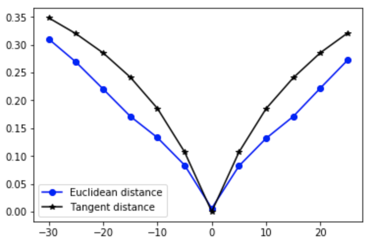
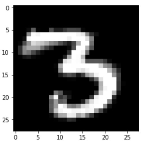
We can see that the Tangent distance are relatively more robust to rotations. Also, with the tangent vector $L$, we can simply achieve the rotation of an image $x$ by adding $\beta L$ where $\beta$ is some constant that determines how much rotation is performed:

p = rotation_deritavtive(x)
p = p.reshape(28, 28)
beta = 5
p = x*255 + beta*p*255

img = Image.fromarray(p)
img = img.convert('RGB')
imshow(img)

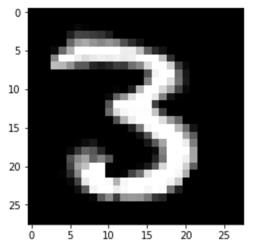
And setting $\beta = -5$ will cause the image to rotate right:

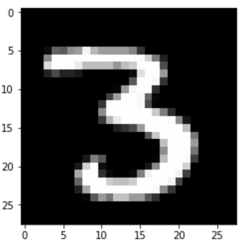
While the original image looks like this:

img = Image.fromarray(x*255)
img = img.convert('RGB')
imshow(img)

How is the tangent distance incorperated in kernel machines? For a tangent distance kernel using the Guassian kernel function: $k(x, x’) = exp(-\frac{1}{2 \epsilon^2} {\lVert x-x’ \rVert}^2)$, just simply replace the Euclidean distance $\lVert \cdot \rVert$ with the tangent distance: $d_{MN}(x, x’)$. Haasdonk et.al. showed that a tangent distance kernel machine with seven tangent directions: x,y-translation, scaling, rotation, line thickening and two hyperbolic transformations achieved $2.4%$ error rate on USPS digits dataset, where human performance is $2.5\%$ error rate.

Thank you for reading!