Learning with Invariances via RKHS

In the previous post I introduced the concept and properities of Reproducing Kernel Hilbert Space(RKHS). In this post, I will introduce how to construct RKHS from a kernel function and build learning machines that can learn invariances encoded in the form of bounded linear functionals on the constructed RKHS.

Given a learning problem, suppose the features of training examples lie in a domain $\mathcal{X}$. A function $k: \mathcal{X} \times \mathcal{X} \to \mathcal{R}$ is called a positive semi-definite kernel if the $\forall l \in \mathcal{N}$ and $\forall x_1, x_2, \dots, x_l$ the $l \times l$ gram matrix it produces: $K[i, j] := k(x_i, x_j)$ is symmetric PSD.

Therefore, given a kernel function $k$, we can constructing a RKHS this way: let $\mathcal{H}$ be a set of all finite linear combinations of functions in ${ k{x, \cdot}, x \in \mathcal{X} }$, that is, ${ k{x, \cdot}, x \in \mathcal{X} }$ span the entire $\mathcal{H}$. Define an inner product on $\mathcal{H}$ as $\langle f, g \rangle = \sum_{i=1}^p \sum_{j=1}^q \alpha_i \beta_j k(x_i, y_j)$ where $f(\cdot) = \sum_{i=1}^p \alpha_i k(x_i, \cdot)$ and $g(\cdot) = \sum_{j=1}^p \beta_j k(y_j, \cdot)$. Let $\mathcal{H}$ also be complete under the inner product $\langle \cdot, \cdot \rangle$, then $\mathcal{H}$ is an RKHS induced by kernel function $k$. For any $f \in \mathcal{H}$, the reproducing properity states that $f(x) = \langle f, K(x, \cdot) \rangle$.

Recall that a functional maps from a vector space to $\mathcal{R}$. We now show that a functional on RKHS is bounded. Let $\mathcal{H}$ be a RKHS induced by a kernel $k$ defined on $\mathcal{X}^2$. Then $\forall x \in \mathcal{X}$, the linear functional $T: \mathcal{H} \to \mathcal{R}$ defines as $T(f) = \langle f, k(x, \cdot) \rangle = f(x)$ is bounded since $\mid \langle f, k(x, \cdot) \rangle \mid \leq \lVert k(x, \cdot) \rVert \cdot \lVert f \rVert = k(x, x)^{\frac{1}{2}} \lVert f \rVert$ by Cauchy-Schwarz inequality.

Let’s now look at Riesz representation theorem. Riesz representation theorem says that for a linear functional $L$ on a Hilbert space $\mathcal{H}$, it’s evaluation of a member of $\mathcal{H}$ can be represented as a inner product: $L(f) = \langle f, z \rangle$ where $z$ is the representer of the funcional and $z \in \mathcal{H}$. $z$ also has norm: $\lVert z \rVert = \lVert L \rVert$ and is uniquely determined by $L$.

For example, let $\mathcal{H}$ be an RKHS induced by a kernel $k$, for any functional $L$ on $\mathcal{H}$, the representer $z$ can be constructed as $z(x) = \langle z, k(x, \cdot) \rangle$ $\forall x \in \mathcal{X}$.

Now, let’s define a semi-supervised learning problem and see how the framework applies to this learning problem. In semi-supervised learning, we have some labeled data and a lot of unlabeled data and we wish to learn a classifier with high accuracy, robustness and good generalization. This problem comes up a lot in learnings where labeled data are expensive to obtain. To define a loss function for optimization, let $(x_1, y_1), \dots, (x_l, y_l)$ be the set of labeled data, and let $\mathcal{l_1}(f(x), y)$ be a convex loss function (e.g. logistic loss, hinge loss and squared loss). This term will be the penality induced by the labeling function $f$ when $f$ mislabels a $x$.

We also measure how much our target labeling function $f$ disatisfies the invariances constraints, and denote them as $L_{l+1}(f), \dots, L_{l+m}(f)$. For semi-supervised learning problems and a lot of other learning problems as well, to learn a good classifier, we will want to encode our prior belief into the learning problem. One reasonable such prior belief is that the gradients of the labeling function in all directions at each labeled and unlabeld instances are small. That is, $f$ doesn’t change very rapidly around each instance. This is a reasonable since instances belonging to the same class tend to cluster together. This will encourage the optimizer to search for an $f$ whose decision boundary is in a low data density reagion since the $f$ tends to change rapidly around decision boundary($f$ has large gradients near decision boundary). We associate another convex loss function with those linear functionals $\mathcal{l_2}(L_i(f))$, this can be squared loss, absolute loss and $\epsilon$-sensitive loss.

Finally, according to Occam’s razor which can be described as the following philosophical message: A short explanation (that is, a hyphothesis that has a short length) tends to be more valid than a long explanation. We also penalize the complexity of $f$ via the RKHS norm ${\lVert f \rVert}^2$. Now we have the following optimization problem:

Where $\lambda, \nu > 0$. Due to the convexity of $\mathcal{l_1}$ and $\mathcal{l_2}$, the above optimization is convex. We now make the following claim that establishes the form of the optimal solution to the above optimization problem:

Let $\mathcal{H}$ be the RKHS induced by kernel $k$. Let $L_i (i=l+1, \dots, l+m)$ be bounded linear functionals on $\mathcal{H}$ with representers $z_i$, the optimal solution to the above optimization must be in the form of:

Therefore, the parameters $\alpha = (\alpha_1, \dots, \alpha_{l+m})’$ (finite dimensional) can be found by minimizing:

where $f = \sum_{i=1}^l \alpha_i k(x_i, \cdot) + \sum_{i=l+1}^{l+m} \alpha_i z(\cdot)$ and $K[i, j] = \langle \hat{k_i}, \hat{k_j} \rangle$, where $\hat{k_i} = k(x_i, \cdot)$ if $i \leq l$, $\hat{k_i} = z_i(\cdot)$ otherwise.

For bounded linear functionals defined as the gradients of the target labeling function $f$ at point $x_i$ at the $d$-th component of $x_i$, denoted as $L_{x_i, d}$, we denote the representer of $L_{x_i, d}$ as $z_{i, d}$. The calculation of $\langle z_{i, d}, k(x, \cdot) \rangle$ and $\langle z_{i, d}, z_{j, d’} \rangle$ for a Gaussian kernel $k(x, y) = exp(-\frac{1}{2 \epsilon^2} {\lVert x-y \rVert}^2)$ are:

Now, we minimize $(1)$ with hinge loss for $\mathcal{l_1}$ and $\epsilon$-insensitive loss for $\mathcal{l_2}$, the quadratic program can be reformulated into the following dual problem:

$\forall i = l+1, \dots, l+m$ and $j = 1, \dots, l$.

We now experiment our new learning framework on the semi-superivised learning problem on the two moons dataset using only two labeled examples. We first load some necessary packages in Python:

from sklearn.datasets import make_moons
import numpy as np
import matplotlib.pyplot as plt
import matplotlib
from cvxopt import matrix
from cvxopt import solvers
from numpy import linalg as LA

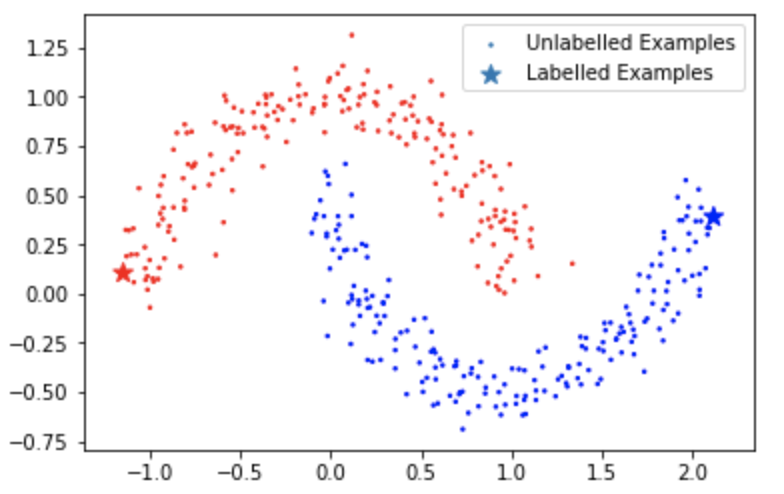
We now load the two moons dataset and label two examples. I chose the two points with maximum and minimum value on the first direction:

seed = 1
X_original, y_original = make_moons(n_samples=400, noise=0.1, random_state=seed)
y_original[y_original == 0] = -1
d = X_original.shape[-1]

#X_train, X_test, y_train, y_test = train_test_split(X, y, test_size=0.2, random_state=seed)
max_idx = list(X_original[:, 0]).index(max(X_original[:, 0]))
min_idx = list(X_original[:, 0]).index(min(X_original[:, 0]))

#idx = list(range(X_original.shape[0]))
#idx = list(np.random.randint(low=0, high=X_original.shape[0]-1, size=int(X_original.shape[0]*0.1)))
idx = [max_idx, min_idx]
X_lab = X_original[idx]
y_lab = y_original[idx]

mask = np.ones(X_original[:, 0].shape, bool)
mask[idx] = False
X_unlab = X_original[mask]
y_unlab = y_original[mask]

X = np.concatenate((X_lab, np.repeat(X_original, d, axis=0)))
y = np.concatenate((y_lab, np.repeat(y_original, d, axis=0)))

colors = ['red','blue']
plt.scatter(X_unlab[:, 0], X_unlab[:, 1], c=y_unlab, cmap=matplotlib.colors.ListedColormap(colors), s=2)
plt.scatter(X_lab[:, 0], X_lab[:, 1], c=y_lab, cmap=matplotlib.colors.ListedColormap(colors), marker='*', s=100)
plt.legend(['Unlabelled Examples', 'Labelled Examples'])

The dataset looks like this:

Now we defined the calculations of $\langle z_{i, d}, k(x, \cdot) \rangle$ and $\langle z_{i, d}, z_{j, d’} \rangle$ as defined in (4) and (5) as well as the Gaussian kernel:

sigma_default = 0.1

def gaussian(x1, x2, sigma=sigma_default):
    return np.exp(-1/(2*sigma**2) * LA.norm(x1 - x2, axis=-1)**2)

def z_xij_gaussian(xi, x, j, sigma=sigma_default):
    return 1/(sigma**2) * (x[j] - xi[j]) * gaussian(xi, x, sigma=sigma)

def z_xij_xpq_gaussian(xi, xp, j, q, sigma=sigma_default):
    if j != q:
        return -1/sigma**4 * (xi[j] - xp[j]) * (xi[q] - xp[q]) * gaussian(xi, xp, sigma=sigma)
    else:
        return 1/sigma**4 * (sigma**2 - (xi[j] - xp[j])**2) * gaussian(xi, xp, sigma=sigma)

and then use those functions to construct the matrix used in the optimization (6):

l = X_lab.shape[0]
dim = X.shape[0]
K = np.zeros((dim, dim))
for i in range(dim):
    for j in range(dim):
        if i < l and j < l:
            K[i, j] = gaussian(X[i], X[j])
        elif i >= l and j < l:
            idx = i % d
            K[i, j] = z_xij_gaussian(X[j], X[i], idx)
        elif i < l and j >= l:
            idx = j % d
            K[i, j] = z_xij_gaussian(X[i], X[j], idx)
        else:
            idx1 = i % d
            idx2 = j % d
            K[i, j] = z_xij_xpq_gaussian(X[i], X[j], idx1, idx2)

We now construct the necessary matrices used in the quadratic programming solver CVXOPT, notice we are using Gaussian kernel with $\sigma = 0.1$, $\epsilon=0.001$ for the $\epsilon$-insensitive loss and $\rho_1 = 1$ and $\rho_2 = 1$:

l = X_lab.shape[0]
Dim = l + (dim-l)*d
length = dim - l
Q = np.zeros((Dim, Dim))
Q[l:l+length, l:l+length] = K[l:, l:]
Q[l:l+length, l+length:] = -K[l:, l:]
Q[l+length:, l:l+length] = -K[l:, l:]
Q[l+length:, l+length:] = K[l:, l:]

M = np.zeros((Dim, Dim))
M[:l, :l] = np.outer(y_lab, y_lab) * K[:l, :l]
G = M + Q

G[l:l+length, :l] = -K[l:, :l]
G[l+length:, :l] = K[l:, :l]
G[:l, l:l+length] = K[:l, l:]
G[:l, l+length:] = -K[:l, l:]

Y = np.ones((Dim, Dim))
Y[l:, :l] = np.tile(y_lab, [Dim-l, 1])
Y[:l, l:] = np.tile(y_lab, [Dim-l, 1]).T
P = G * Y

epsilon = 0.001
rho1 = 1
rho2 = 1
q = np.zeros((Dim, 1))
q[:l] = -1
q[l:] = epsilon

N = np.vstack((np.eye(Dim)*(-1.),np.eye(Dim)))
constraint = np.zeros((Dim))
constraint[:l] = 1 / (2*rho1)
constraint[l:] = rho2 / (2*rho1)
h = np.hstack((np.zeros(Dim), constraint))

P = matrix(P)
q = matrix(q)
G = matrix(N)
h = matrix(h)

# run solver
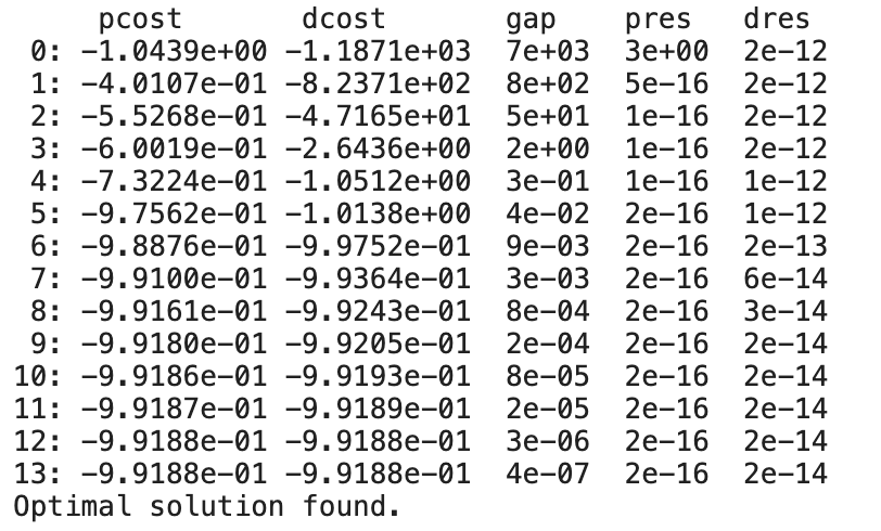
sol = solvers.qp(P, q, G, h)
vals = np.array(sol['x'])

As we can see from the outputs by the solver, the quadratic program is solved very efficiently and reaches a global optimum:

we now collect the optmization results and define the classification function based on the form of the optimal solution:

beta = vals[0:l]
alpha_prime = vals[l:l+length]
alpha = vals[l+length:]
a = alpha_prime - alpha

sup_vec_idx = np.union1d(np.argwhere(np.logical_or(alpha_prime > 1e-4, alpha_prime < -1e-4)), np.argwhere(np.logical_or(alpha > 1e-4, alpha < -1e-4)))

def classify(x, beta, a, sup_vec_idx):
    val = 0
    for xi, b, y in zip(X_lab, beta, y_lab):
        val += b * gaussian(xi, x) * y
    X_tmp = np.repeat(X_original, d, axis=0)
    for idx in sup_vec_idx:
        j = idx % d
        val += a[idx] * z_xij_gaussian(X_tmp[idx], x, j)
    return np.sign(val)

The classification is computing the linear combinations of kernel functions and bounded linear functionals. Now let’s take a look at the learning outcome and the decision boundary:

max_x = max(X[:, 0])
min_x = min(X[:, 0])
max_y = max(X[:, -1])
min_y = min(X[:, -1])

xline = np.linspace(min_x-0.1, max_x+0.1, 100)
yline = np.linspace(min_y-0.1, max_y+0.1, 100)

cartesian = []
for x in xline:
    for y in yline:
        cartesian.append((x, y))
cartesian = np.array(cartesian)

predictions = []
for pair in cartesian:
    predictions.append(classify(pair, beta, a, sup_vec_idx))
    
predictions = np.array(predictions)

colors = ['yellow','white']
colors1 = ['red','blue']
plt.scatter(cartesian[:, 0], cartesian[:, 1], c=predictions.squeeze(), cmap=matplotlib.colors.ListedColormap(colors), s=2)
plt.scatter(X_original[:, 0], X_original[:, 1], c=y_original, cmap=matplotlib.colors.ListedColormap(colors1), s=2)

The decision boundary looks like this:

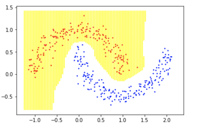
Which is a perfect and clean sepration. This learning framework can be applied to supervised learning problems and encode different prior beliefs as bounded linear functionals on an RKHS. By minimizing gradients of target labeling function at data points, we can produce a smooth classifier. Smoothness in classifiers has a lot of benefits including robustness to adversarial examples.

The Jupyter notebook for the code can be found here.

Thank you for reading!